Martingale Strategy: Complete Guide to Doubling-Down, Probability Math, and Historical Blowups

The Martingale strategy is a money-management method that originated in 18th-century French casinos. Its core logic is simple: every time you lose, you double your next bet, repeating until you win. In forex and CFD trading, it shows up as repeatedly doubling down (averaging) as price moves against you, pulling the average cost closer so that even a small bounce turns the whole position profitable. In theory you “always win if your capital is infinite” — but real capital is finite: a losing streak makes position size and margin requirements balloon exponentially, so a one-way market can wipe you out in a single liquidation. This is the mathematical inevitability of Gambler's Ruin.

“If you keep doubling after a loss, you’ll always win it back eventually.” The Martingale strategy is the method almost every beginner runs into — and the one most likely to be misunderstood. Its intuitive logic has lured countless forex, CFD, and crypto traders. But can a strategy born in the gambling world really work in modern financial markets?

This article starts from first principles and breaks down, step by step, how Martingale actually behaves in live trading. We explain why it looks perfect yet hides a fatal risk, and offer practical risk-management advice so you can make a rational choice once you understand the truth.

1. What Is the Martingale Strategy? Core Logic and Principles

The Martingale Strategy was born in 18th-century France, where it was first applied to simple "coin-toss" games and "1:1 odds" wagers. Its operating logic is extremely pure: every time you suffer a loss, you double the stake on the next round until you win. The moment you win, you immediately reset the stake to the initial amount and begin a brand-new cycle.

Example: Martingale in a Coin-Toss Game

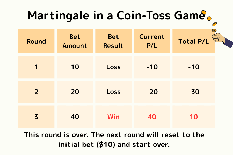
Suppose you take part in a game of guessing whether a coin lands heads or tails, where each correct guess pays a reward equal to your bet.

Final result: Even though you lost the first two rounds, the profit from the third round (40) minus the losses from the first two rounds (30) still leaves you with a net profit of USD 10, which is exactly your original bet amount.

What happens after a win?: Once a cycle ends in a win (that is, you recover everything and earn the profit equal to your initial bet), you immediately reset the stake back to the original USD 10 and start a brand-new round of betting. This way, each time you complete a "loss → double → win" cycle, you lock in a small fixed profit (USD 10 in this example), then start over, avoiding overexposing your gains to subsequent risk.

In theory, as long as your capital is large enough to support an unlimited number of doublings, you will eventually win back all your losses and earn that first initial reward.

1.3 Mathematical Origins: From 18th-Century French Casinos to Paul Lévy's 1934 Martingale Theory

The prototype of Martingale can be traced back to the 18th-century French casino—originally a coin-game system of "double down again after every loss." However, the true mathematical foundation of this strategy was not established until the 20th century:

Year	Scholar	Contribution
1934	Paul Lévy (France)	Introduced the modern concept of the "martingale" into probability theory
1939	Jean Ville (France)	Formally named the "martingale" and extended it to continuous-time martingales
1956	Joseph Doob (USA)	The martingale convergence theorem, laying the foundation of modern probability theory

1.4 The Gambler's Ruin Theorem: Why "Guaranteed to Win" Becomes "Guaranteed to Lose"

Modern probability theory has clearly proven a cruel fact: a gambler with finite capital, facing an opponent with infinite capital (such as a casino or the market), will almost certainly go bankrupt over long-term repeated gambling—even if every single round is a "fair" 50/50 bet.

Consecutive losses N	Probability P(N) = 0.5^N	Required bet amount (initial USD 10)
5	3.13%	USD 160
10	0.098%	USD 5,120
15	0.003%	USD 163,840
20	0.0001%	USD 5,242,880

The probability of 10 consecutive losses is only 0.098%, which seems rare, but it occurs roughly once in every 1,000 repetitions—and the loss from that single event will be hundreds of times greater than the accumulated profits. This is the mathematical essence of Gambler's Ruin.

2. How the Martingale Strategy Works in Financial Markets

In financial trading (such as forex or CFDs), the application of the Martingale Strategy is far more complex than in a casino; it is usually viewed as an extreme form of "averaging down cost" management.

Operation: Phased Entry and Dynamic Averaging Down

When a trader opens a buy position in the forex market (for example, 0.1 lots) and the price keeps falling, the Martingale trader will not choose to stop-loss and close the position; instead, after the price falls by a certain interval, they add a larger size (such as 0.2 lots). If the price continues to drop, they add 0.4 lots, then 0.8 lots, and so on.

The purpose of this approach is to continuously pull the overall "holding cost" closer to the current price. Once the market shows even the smallest rebound, the average cost of the entire group of orders can be covered, achieving an overall profitable exit.

Mechanism: The Extreme Pursuit of an Average Entry Price

In financial markets, this is called "averaging down." By exponentially increasing the position size, the trader dramatically reduces the retracement needed to "turn a loss into a profit."

As long as the market does not move forever in a single direction without turning back, in theory this trade can ultimately end in profit.

2.3 Martingale vs. Grid Trading vs. Averaging Down (Nampin)

In practice, Martingale is often confused or used together with three concepts:

Strategy	Add-on Logic	Danger Level	Typical Tools
Martingale	Double the position after every loss (2x, 4x, 8x…)	Extremely high	Forex EAs, casinos
Grid Trading	Add equal amounts within a preset price range	High	Forex EAs, algorithmic trading
Averaging Down / Nampin	Add discretionary amounts on declines to lower average cost	Medium–High	Long-term stock investing
Dollar Cost Averaging	Invest equal amounts regularly, regardless of price	Low	Fund SIPs, pensions

On MT4 / MT5 platforms, 60–80% of commercial EAs adopt Martingale or grid logic, which is also the main reason the FX EA market has long exhibited the phenomenon of "double your money in a year, wiped out in one go."

2.4 How Different Jurisdictions Regulate Martingale EAs

Region	Key Rule	Impact on Martingale
USA	NFA Rule 2-43(b) (2009) FIFO rule and hedging ban	Completely breaks the logic of most Martingale EAs
Japan	FSA maximum leverage of 25x from 2010/8/1; mandatory loss cut from 2011/8/1	Speeds up the exhaustion of margin from consecutive doublings
EU	ESMA retail leverage caps from 2018/8: 30x for major pairs, 20x for minor pairs, 2x for crypto	Clearly compresses the room for Martingale operations
UK	FCA 2019 retail leverage cap of 30x + CFD warning labels	Same restrictions as ESMA
Canada	CIRO max leverage 33:1	Same as above

The 2015/1/15 Swiss franc shock (SNB abandoning the exchange-rate floor): EUR/CHF plunged 3,947 pips within minutes; Alpari US / Alpari Japan went bankrupt, and FXCM survived only after receiving a USD 300M emergency loan. This event revealed that "in a black-swan one-way market, any add-on strategy can go to zero in an instant"—even the most conservative grid trading cannot escape unscathed.

3. Why Do Beginners Love Martingale? Two Core Advantages

For newcomers just getting into trading, the Martingale Strategy carries an extremely strong psychological allure, because it appears to solve the two hardest problems in trading: the fear of loss and the difficulty of forecasting.

Advantage 1: It Creates a Very High Apparent Win Rate

In range-bound markets, the Martingale Strategy displays an astonishing frequency of profits.

Because every adverse price move is met with doubling the bet to pull the cost closer, most orders ultimately end up being settled at a profit.

For beginners, this "winning money almost every day" data performance provides a huge sense of achievement and psychological security, making the account balance show a steadily rising curve under normal market conditions.

Advantage 2: It Significantly Lowers the Barrier to Market Forecasting

Most trading strategies require investors to have the ability to precisely judge trends, entry points, and exit points, but the Martingale Strategy simplifies trading logic into "waiting for a pullback."

Traders do not need to judge the long-term bullish or bearish direction of the market, nor do they need to pinpoint precise turning prices; as long as the market does not move forever in a single straight line without turning back, in theory they can obtain a final winning point through continuous averaging down.

This characteristic of not requiring a deep foundation in technical analysis makes it a top choice for many beginners seeking a "shortcut to trading."

4. Fatal Flaws: The Three Real Risks of the Martingale Strategy

Although the theory is beautiful, in reality capital is not infinite, which makes the Martingale Strategy extremely dangerous in real financial-market practice.

Risk 1: Exponential Capital Inflation and Margin Pressure

The power of doubling is staggering. To observe the risk more intuitively, let us assume a trader starts at 0.01 lots and adds positions at a fixed price interval (for example, every 50-point drop) (excluding spread and interest costs, ignoring the amplifying effect of additional price volatility on losses, and focusing solely on the doubling of lot size itself):

Round	Lot added this round	Cumulative lots (total position)	Position-size inflation multiple
1	0.01	0.01	1x
2	0.02	0.03	3x
3	0.04	0.07	7x
4	0.08	0.15	15x
5	0.16	0.31	31x
6	0.32	0.63	63x
7	0.64	1.27	127x
8	1.28	2.55	255x
9	2.56	5.11	511x
10	5.12	10.23	1,023x

From the table, you can see that after just 10 rounds of consecutive losses, your total position size balloons from the original tiny 0.01 lots to 10.23 lots, inflating by more than 1,000x.

This is not merely a matter of book losses; more importantly, your account must provide a huge "advance payment (margin)" to support these orders. Once the market produces a one-way move and your capital cannot keep up with the pace of doubling, the system will collapse in an instant.

Risk 2: The Final Judgment of Forced Liquidation

In financial markets, when your available margin is insufficient to support the losses and margin requirements, the broker will execute a forced liquidation (Loss Cut). For Martingale users, this usually means a "one-shot blowup."

Because in a one-way directional market (such as a black-swan event), the market may exhaust all your capital before it turns back.

Risk 3: The Extreme Disproportion Between Drawdown and Profit

To earn a mere USD 10 of initial profit, a Martingale trader may have to endure thousands or even tens of thousands of dollars in floating losses (drawdown). This risk-reward ratio of "betting your life for a penny" is extremely inconsistent with investment logic over the long run of capital management.

4.4 Historic Blowup Case Studies: When Martingale Logic Destroys Institutions

Martingale is not a trap only retail traders step into. Several of the largest institutional collapses in financial history were, at their core, "adding positions after losses to lower the average cost"—that is, a variant of Martingale:

Case 1: LTCM 1998 (The Epic Failure of Nobel Laureates)

Long-Term Capital Management was founded by John Meriwether (1994), and its partners included 1997 Nobel laureates in Economics Myron Scholes and Robert C. Merton.

• Capital structure: Shareholders' equity USD 4.8B → borrowings USD 125B+ + derivatives notional USD 1T
• Leverage ratio: Initial 25:1 → end of 1998/8 50:1 → third week of September 130:1
• Fatal behavior: In late 1997 it returned capital to investors while maintaining the same positions (numerator decreases, denominator unchanged → leverage automatically amplifies, i.e. "doubling down" in the mathematical sense)
• Result: Losses of USD 4.6B from July to September 1998, with a single-month loss of 44% in August; the New York Fed brokered an emergency USD 3.6B rescue by 14 banks
• Lesson: Even an academically backed "convergence arbitrage model" can have all positions fail simultaneously when correlations spike under stress (tail correlation)

Case 2: Amaranth Advisors 2006 (USD 6.6B Vanished in a Week)

• Protagonist: Brian Hunter, who ran natural gas spread trades
• Loss: A single-week loss of USD 6.6B in September 2006 (the largest hedge fund collapse in history at the time)
• Behavior pattern: After the natural gas calendar spread reversed, he insisted on adding positions, exhausting the liquidity buffer

Case 3: Archegos 2021 (The Largest Family-Office Blowup of the 21st Century)

• Protagonist: Bill Hwang's USD 10B family office
• Method: Through Total Return Swaps (TRS), hidden ~20:1 leverage across multiple prime brokers (Nomura provided 4x the leverage of a typical long/short fund)
• Doubling-down evidence: On 2021/3/23, Hwang directed the additional purchase of ~USD 1 billion of already-declining positions such as ViacomCBS to "support the price" (later deemed market manipulation by the SEC)
• Collapse: On 2021/3/26, margin calls failed → USD 20B in fire sales
• Chain losses: Nomura USD 2 billion loss, Credit Suisse USD 5.5 billion loss (which later collapsed in March 2023 and was acquired by UBS, with this event being one of the main causes)
• 2024/11 verdict: Hwang was sentenced to 18 years in federal prison on serious felony charges

Case 4: Barings Bank 1995 (A 233-Year-Old Bank Buried by One Man)

• Protagonist: Nick Leeson of the Singapore branch
• Method: After losses, he kept adding to Nikkei 225 futures positions in an attempt to win it all back
• Result: £827M (about USD 1.4B) loss; Barings Bank went bankrupt and was acquired by ING for a symbolic £1

Case 5: VIX ETN / XIV 2018/2/5 ("Volmageddon")

• Instrument: VelocityShares Daily Inverse VIX ST ETN (XIV)
• Result: A single-day drop of 96%, wiping out USD 1.9B in AUM (before liquidation); its underlying strategy (selling VIX futures) was essentially an implicit Martingale exposure of "collecting small premiums → blowing up when a tail event hits"

4.5 The Common Pattern: Why Do Institutions Fall into the Martingale Trap?

• Belief bias: "Mean reversion" and "oversold rebound" are taken as absolutes
• Financing-incentive mismatch: Performance fees encourage increasing risk in pursuit of big wins
• Liquidity illusion: Markets that flow smoothly in normal times can vanish in an instant under stress (volatility gap)
• Underestimating correlation: Diversified positions move in the same direction simultaneously during black-swan events (tail dependence)

5. Practical Advice: How to Improve Martingale to Reduce Risk

If you still want to try this strategy in your trading, you must carry out a strict "detoxification" improvement rather than blindly doubling.

Improvement 1: Set a Maximum Number of Add-on Layers and a Hard Stop-Loss

Never add positions an unlimited number of times. For example, set a rule that you "add at most up to the 5th layer," and if the market still does not turn back, you must admit failure and close the entire position. This preserves the residual value of your account and prevents a single mistake from knocking you out completely.

Improvement 2: Adjust the Doubling Factor (Diluted Martingale)

You do not have to strictly multiply by 2 every time. Adopting a growth ratio of 1.2x or 1.5x (such as 0.1 / 0.12 / 0.15 ...) can significantly slow down the pace of position inflation, thereby buying more survival time and room for market fluctuations.

Improvement 3: Combine with Filter Indicators

Do not casually launch the strategy at just any position. We recommend combining it with the RSI overbought/oversold indicator, or support and resistance levels and other technical analysis. Only consider adding positions when the market shows a strong probability of a pullback; this can greatly increase the success rate of the strategy and reduce ineffective averaging down.

5.4 Anti-Martingale and the Kelly Criterion: The Mathematically Correct Solution

The Kelly Criterion is the mathematical opposite of Martingale. Proposed by Claude Shannon (the father of information theory) and John L. Kelly Jr. (Bell Labs, 1956), it indicates the optimal betting fraction that "maximizes the long-run logarithmic growth rate":

$$f^* = \frac{bp - q}{b}$$

where $b$ = odds, $p$ = win rate, $q$ = loss rate ($q = 1-p$).

Example: a fair game (odds $b$ = 1:1) + a 55% win rate: $$f^* = \frac{1 \times 0.55 - 0.45}{1} = 0.10$$

That is, bet 10% of your capital each time (rather than going all-in or doubling).

Edward Thorp's Legendary Empirical Record

Edward Thorp (author of Beat the Dealer, 1962, and the first mathematician to systematically beat Blackjack in casinos) applied the Kelly Criterion to investing:

• Princeton-Newport Partners (1969-1988): 19 years of 19.1% annualized return (after fees)
• One of the earliest quant hedge funds in history, opening the quantitative tradition later carried on by the likes of Jim Simons's Renaissance Technologies

Practical Strategy: Fractional Kelly

Full Kelly is extremely sensitive to short-term losses (although optimal in the long run), so institutions often use "Half Kelly ($f^/2$)" or "Quarter Kelly ($f^/4$)":

Kelly fraction	Expected annualized return	Short-term maximum drawdown (psychological pressure)
Full Kelly	100%	Extremely high (can reach 50%+)
Half Kelly	75%	Medium (25-30%)
Quarter Kelly	44%	Low (15%)

The spirit of Anti-Martingale is to "add size when winning, cut size when losing," which is the complete opposite of Martingale. Stanley Druckenmiller (former chief strategist of George Soros's Quantum Fund) has publicly stated that he has long used the anti-Martingale mode: adding positions once a trend is established, and immediately cutting size when signs of reversal appear.

5.5 Kelly Criterion vs. Martingale Strategy Comparison

Dimension	Martingale	Kelly Criterion (Anti-Martingale)
Betting basis	The result of the previous round	Expected win rate and odds
After a loss	Double up	Maintain or reduce
After a profit	Reset to initial	Scale up by the Kelly fraction
Theoretical basis	Casino intuition	Information theory (Shannon 1956)
Probability of ruin	Finite capital → inevitable	Under positive expected value → minimized
Empirical record	LTCM, Archegos, Amaranth, Barings all failed	Thorp: 19.1% over 19 years; Buffett uses similar logic

6. Frequently Asked Questions (FAQ)

Q1: Is the Martingale strategy suitable as a primary trading system?

Generally not. It is better used as a very small part of an overall system — an auxiliary tool for specific range-bound conditions. Betting your entire account on Martingale almost always ends in a blowup.

Q2: Is running Martingale with an EA (automated script) safer?

No. A computer can add to positions more precisely, but it cannot foresee black swan events. Many blown accounts came from setting an EA and leaving it unattended — in a one-way trend, the bot quickly drains your margin.

Q3: How much capital does an account need to run Martingale?

There is no fixed answer, but the principle is that your initial position must be "negligible" relative to account equity. For a $10,000 account, the initial position should be smaller than 0.01 lots, leaving room to absorb repeated averaging-down in extreme conditions.

Q4: What is the "Anti-Martingale strategy"?

Anti-Martingale is a class of money-management strategies that cut size on losses and add size on wins. Its most classic form is the Paroli system: scale up during winning streaks and reset to the base stake after a loss — controlling downside while maximizing gains during streaks.

7. Conclusion: Martingale Is a Double-Edged Sword

The Martingale Strategy is perfect in mathematical logic, but extremely fragile in the real financial world. It exploits the psychological advantage of "averaging down" while ignoring the cruel reality of finite capital and extreme one-way markets.

For investors, the best protection is to build correct risk awareness. Remember: in financial trading, surviving long is more important than winning fast. If you intend to use Martingale, be sure to keep it within an affordable risk range, and always be prepared to stop out at any time for that extreme market that "just won't turn back."

---

Further Reading

• What Is a CFD?
• What Is Averaging Down?
• What Is a Stop Loss?
• What Is a Black Swan Event?
• What Is Loss Cut (Forced Liquidation)?

---

Primary Sources (by Category)

• Academic theory: Paul Lévy (1934) / Joseph Doob martingale convergence theorem (1953) / Kelly Criterion, Bell System Technical Journal (1956)
• Historical cases: LTCM (1998, NY Fed-brokered rescue), Archegos (2021, SEC/DOJ), Barings Bank (1995, Bank of England report)